Giskard + Grafana for Data Drift Monitoring

Introduction

In our previous tutorial, we learned about monitoring data drift using Giskard. This time, we're focusing on how to use Grafana to visualize these data drift results. This tutorial will guide you through setting up Grafana and creating a dashboard to display your data drift test results. If you prefer to learn by doing, you can follow along with the code provided here.

Why Should you visualize Data Drift test results?

Consider this: what speaks louder, rows of numbers in an Excel sheet or a dynamic interactive graph? Visual data interpretations not only make it more intuitive but also speed up the analysis process, especially since we often do it regularly. In this part, we'll discover how a Grafana dashboard not only simplifies the interpretation of data drift results but also offers added functionalities like alerting.

Overview: Main ideas in Data Drift Detection

In this tutorial, we leverage Giskard for conducting drift tests and storing the results in a PostgreSQL database for robust and scalable data management. Grafana will then be used to query this database and visualize the results.

Benefits of using Giskard with Grafana:

• Dynamic Testing with Giskard: Giskard's versatility shines as it allows us to input different `reference dataset` (standard or historical data) and `current dataset`` (new, incoming data), along with the `model`, at runtime. This flexibility is invaluable for periodic testing on production data, enabling us to consistently and automatically run the same test suite on new data batches or updated models.
• Real-Time Insights with Grafana: It not only provides real-time visualization of drift test results but also facilitates team collaboration by allowing us to share insightful dashboards. This is an important aspect of continuously monitoring our models, making it easier to quickly identify and react to any significant changes in the data.

Setting up Grafana dashboard for effective ML Model Drift Detection

We’re taking a slightly different approach for this tutorial by using Python scripts instead of Jupyter notebooks. The reason? It's all about automation and efficiency. With scripts, we can easily schedule recurring tasks using a tool like cron.

Our setup is streamlined using Docker Compose. It's a neat way of bundling all our required services into one manageable package. Let's take a look at our `docker-compose.yml`:

This file outlines three key services:

• db: Our PostgreSQL database, where we'll store all the results from our drift tests.
• adminer: A handy web interface for managing our PostgreSQL database.
• grafana: We’ll use this for creating dashboards to visualize drift test results.

To start the services in the background, use docker-compose up -d. To stop them, run docker-compose stop, and to stop and remove the containers, use docker-compose down.

The `postgres_data` volume ensures data persistence, and two networks, `front-tier` and `back-tier`, manage service connectivity and exposure.

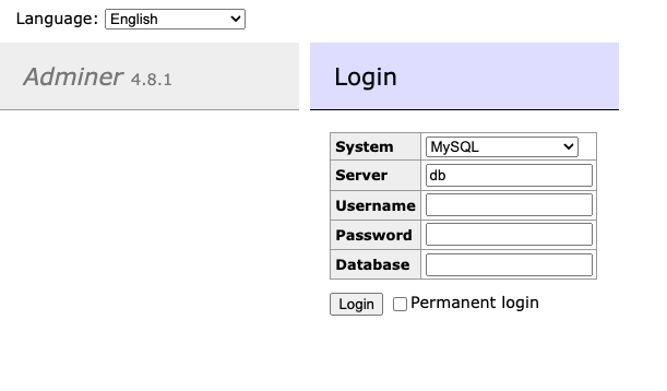
Once up, we can access Grafana at `http://localhost:3000/` (login with username and password both as admin. Next, you'll be prompted to change the password), and Adminer can be accessed at `http://localhost:8080/` (system: PostgreSQL, username: postgres, password: postgres, database: giskard_monitoring).

Note: Login into Adminer after running the `main.py` file in the `src` directory because the database will be created after we run the file at least once. Otherwise, we’ll see an error `Invalid database`.

‍

Directory structure and files

Let's take a look at how we've organized our project for this tutorial. A well-structured directory ensures everything is easy to find and understand.

• config: It contains the configuration files for Grafana. The `grafana_datasources.yaml` file contains the configuration for the PostgreSQL database. The `grafana_dashboards.yaml` file contains the configuration for the dashboard.
• dashboards: Contains the JSON file defining our Grafana dashboard, detailing its layout, panels, and queries.
• data: This is where our reference and raw data (raw_data.parquet) reside, the latter simulating our production data.
• model: It contains the model we'll be using to perform the drift test on the target variable.
• notebook: Contains a Jupyter notebook used for initial experiments and development.
• src: It contains the source code for this tutorial. `db.py` manages database connections, `giskard_drift_test_suites.py` is for creating test suites, and `main.py` orchestrates running these tests and storing results.

Implementing Drift Monitoring with Giskard

In this tutorial, we're utilizing the Bike Sharing Dataset from the UCI Machine Learning Repository. This dataset includes hourly and daily counts of rental bikes between 2011 and 2012 in the Capital bikeshare system, along with weather and seasonal information. We'll be using the daily dataset for this tutorial.

The relevant data for this tutorial are located in the `data` directory. Here, raw_data represents the production data we'll simulate, and reference_data serves as our benchmark. From our previous tutorial, we have a saved model in the model directory, which we'll use to conduct drift tests on the target variable.

Mimicking Production Data

Our approach to emulate production data involves using 100 rows from raw_data to create each batch. This process is repeated five times, resulting in five distinct batches. This method effectively simulates a real-world scenario where new data batches are continuously processed and evaluated for drift.

For illustration purposes, the five batches correspond to five days of production data. However, it's important to note that the frequency of performing drift calculations may vary depending on the specific use case.

Creating the Test Suites for Data Drift Detection

In our `giskard_drift_test_suites.py` file, we have key functions to create and manage our test suites. These suites are essential for detecting data drift in various features of our dataset.

• _check_test Function: This function dynamically selects the appropriate test based on the feature type (numeric or categorical) and dataset size. It uses a prediction_flag to decide if the test should be applied to the target variable.
• test_drift_dataset_suite Function: This function constructs the test suite by calling _check_test for each feature.
• dataset_drift_test Function: Here, we aggregate the results from individual tests to assess the overall drift in the dataset.

Connecting to the Database

In the `db.py` file, we establish our connection to the database using the psycopg library, chosen for its seamless integration with PostgreSQL and its user-friendly interface in Python.

• prep_db function: This function ensures that our database 'giskard_monitoring' and the required table are set up correctly. It first checks if the database exists, and if not, it creates it. Then, it sets up a table for storing our data drift metrics.
• insert_into_db function: This function inserts the results of our drift tests into the database. Storing these results allows us to track and analyze the performance of our models over time.

Main Script

In the main.py file, we bring together all the components of our tutorial. This script is the core of our project, where we run the test suites and store their results in the database.

Setup and Data Preparation

We begin by importing necessary libraries and defining constants. The `raw_data` and `reference_data` are loaded from the data directory, and the model is loaded from the `model` directory.

By wrapping the model into a Giskard Model object and the reference_data into a Giskard Dataset object, we prepare our data and model for the drift tests. The prediction_function is defined for making predictions with the model.

Computing Drift Metrics and Database Interaction

The `compute_drift_metrics` function calculates drift metrics using the test suites defined in `giskard_drift_test_suites.py` and inserts them into the database.

We divide the `raw_data` into 100-row chunks and calculate drift metrics for each chunk. Each chunk represents one day's worth of data on the chart, constituting a single data point. We repeat this process to extract a total of 5 chunks, corresponding to 5 days of data.

Batch Monitoring:

The `batch_monitoring` function orchestrates the overall monitoring process. It connects to the database and performs the drift metric calculations for five data chunks, in line with our simulation approach.

Execution:

To run this script, execute the command python src/main.py from the root directory of the project. This will kickstart the batch monitoring process, performing drift tests and storing results.

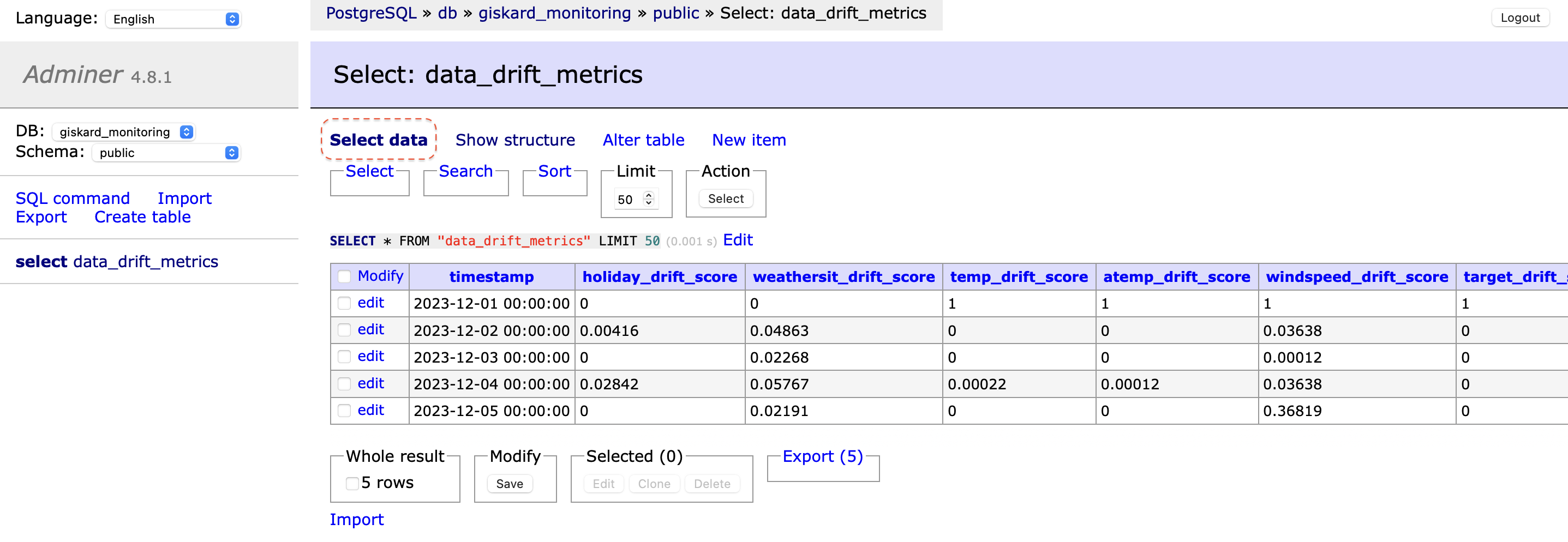
Viewing Data Drift Results:

Once the script has run, the results of the drift tests can be viewed in the database. Access the Adminer portal at http://localhost:8080/, navigate to the `data_drift_metrics` table, and select `Select data` to examine the test outcomes.

Creating the Dashboard for Drift Monitoring

Now that we have our data successfully feeding into Grafana, it's time to bring it all together in a dashboard. This dashboard will serve as a visual representation of our drift metrics, providing an intuitive and insightful view of the evolution of drift over time.

Because the dashboard configuration is stored in the dashboards directory, Grafana will automatically load this configuration when it starts. This means there's no need to create a new dashboard from scratch manually.

When you open Grafana, select `Drift Dashboard` and a dashboard similar to the one depicted in the image below will be shown. This dashboard is a direct result of running the `main.py` script, which executed the drift tests and stored their results in the database. The dashboard queries this data and displays it, allowing you to immediately see the outcomes of the drift tests.

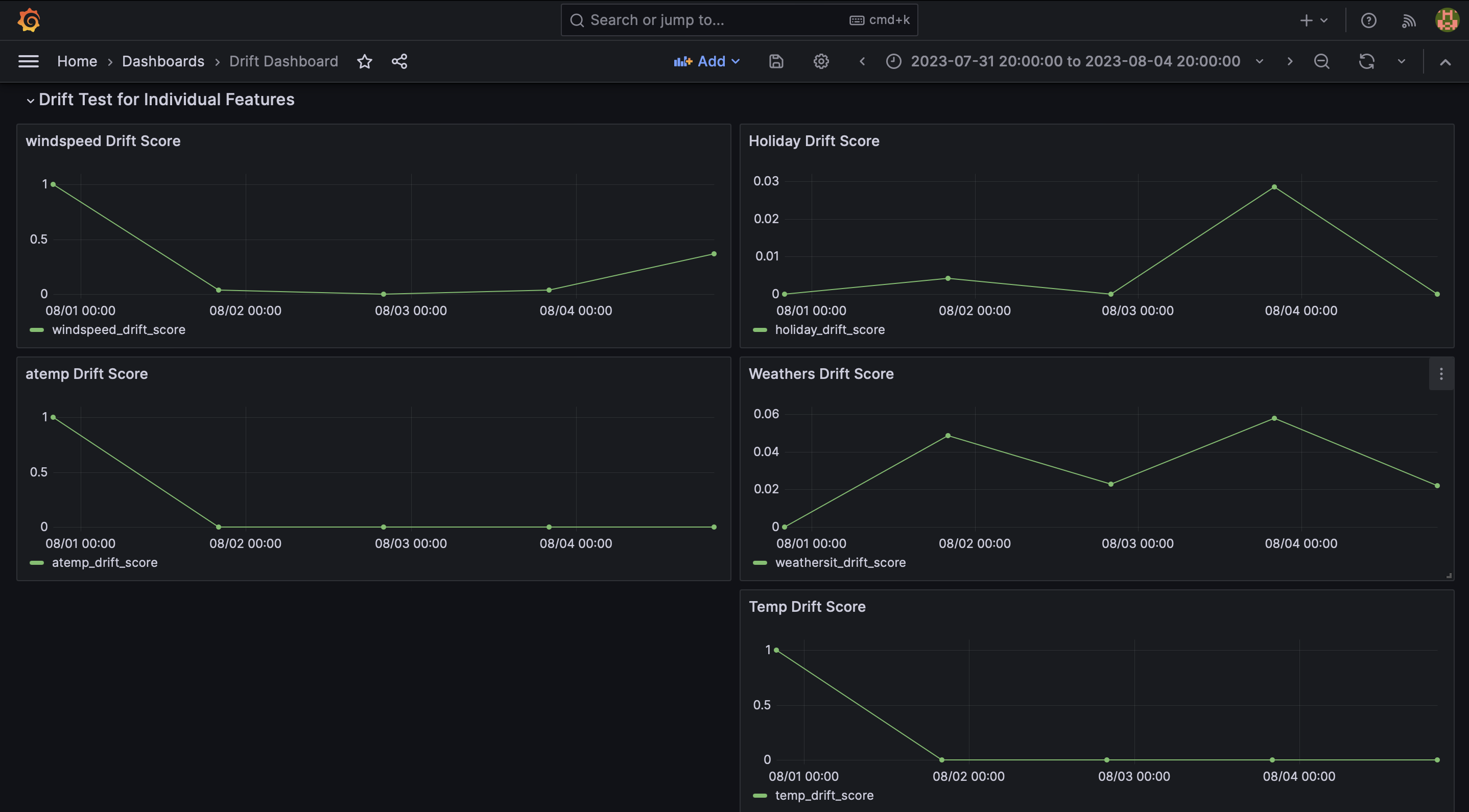
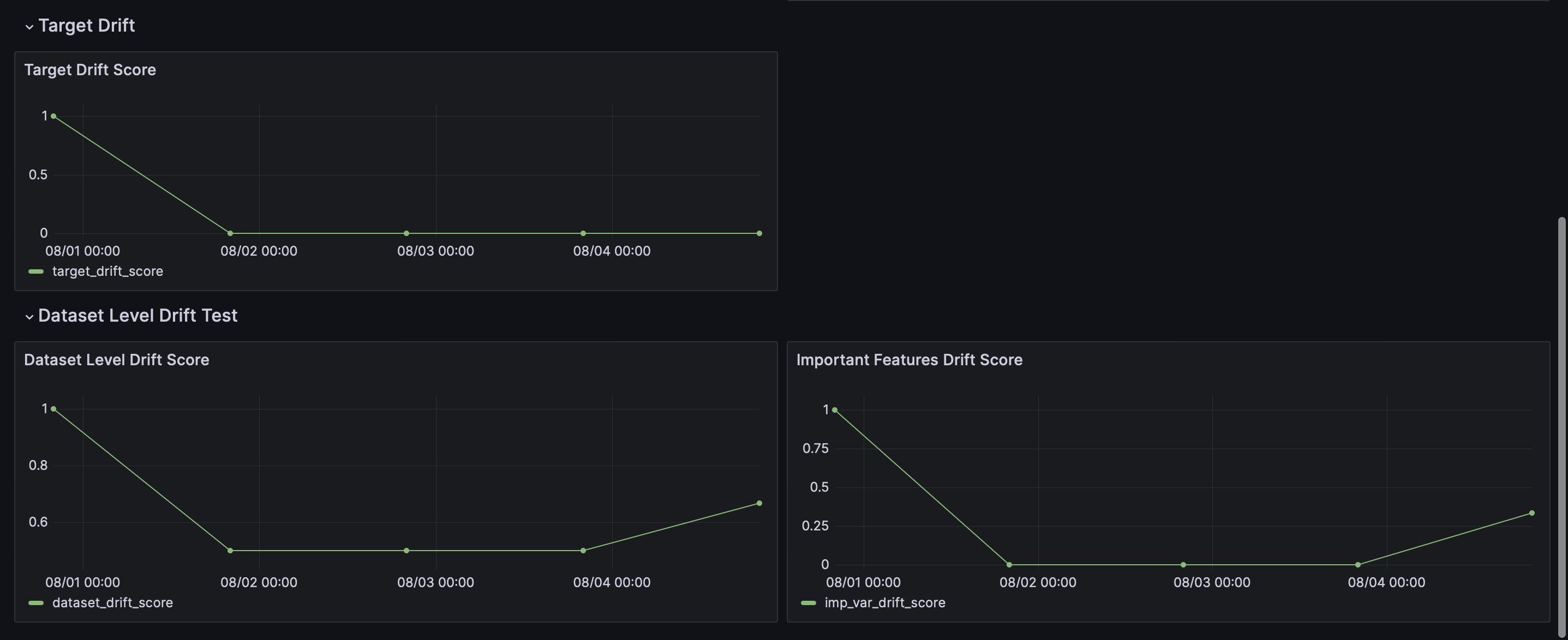
On the x-axis we can observe the timestamp and y-axis value corresponds to the result for each test.

However, for demonstration purposes, we'll walk through creating a basic visualization manually.

Steps to create a ML Model Drift dashboard and add a visualization

1. Accessing Dashboard creation

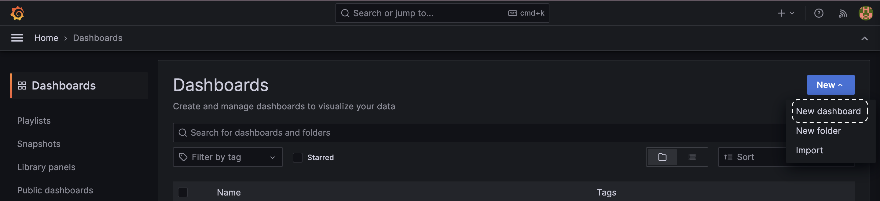
1. Log in to Grafana, open the Menu on the left side of the screen, and click on Dashboards.
2. Select New from the dropdown menu and choose New Dashboard.

2. Adding a Visualization

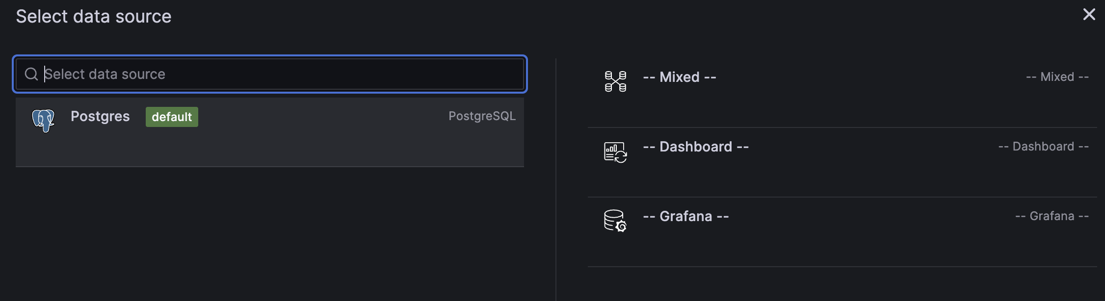
1. Click on Add visualization.

2. Choose PostgresSQL as the data source.

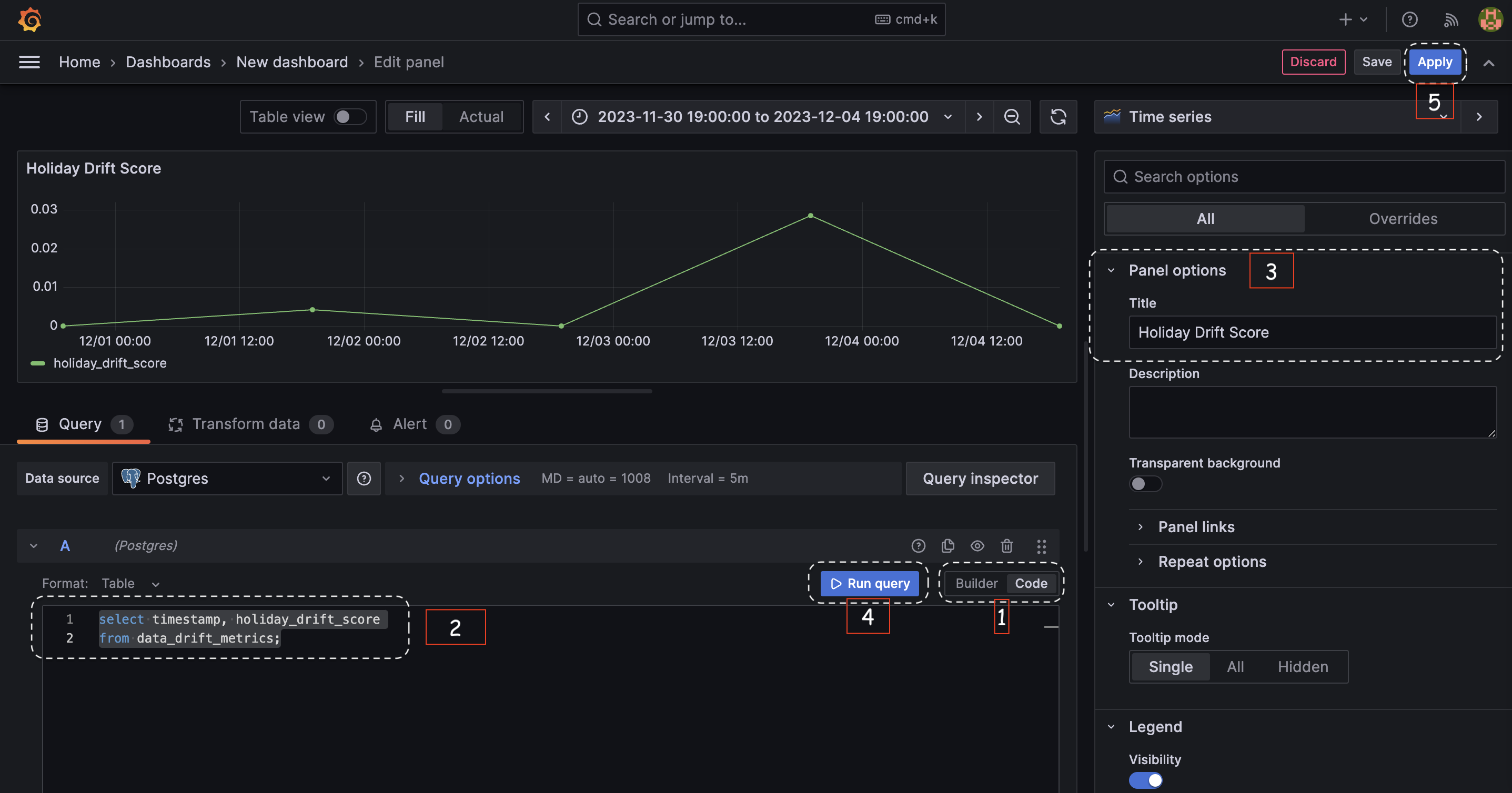
3. In the query editor, select the code option and paste the following SQL query:

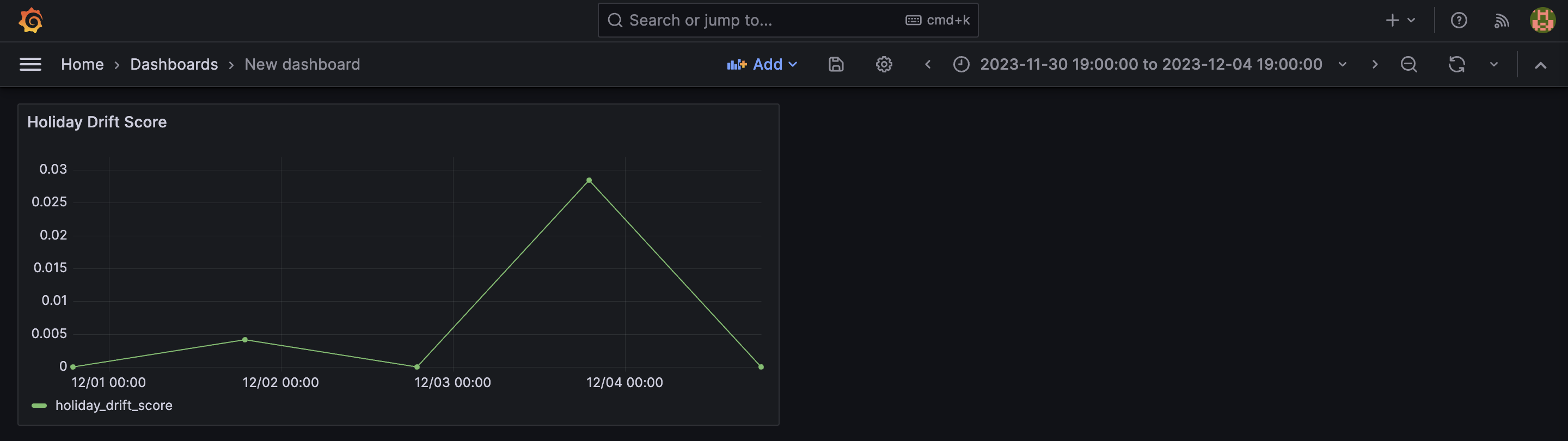
4. In the Panel options, set the Title to Holiday Drift Score.

5. Click on Run query to execute the query and display the results. You may need to click Zoom to data to focus on the most relevant data points.

6. Hit Apply to save the visualization.

3. Saving and Expanding the Dashboard

1. To save the dashboard, click on the save icon (resembling a floppy disk) at the top of the screen.
2. Enter a name for your dashboard and click Save.
3. Repeat the above steps to add more visualizations to your dashboard as needed.

4. Exporting Dashboard Configuration

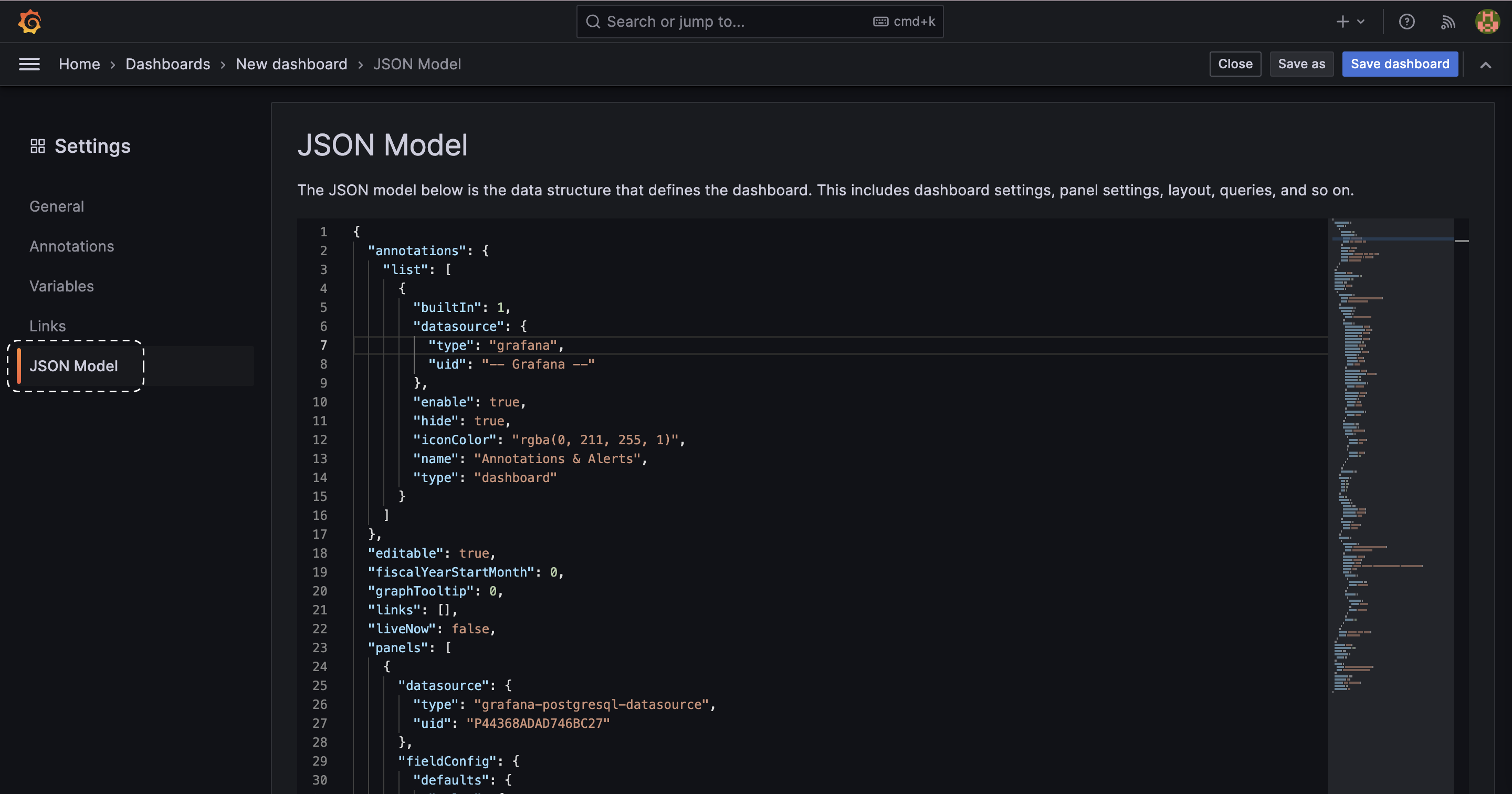
1. To get the JSON model of the dashboard, click on the Dashboard settings icon (resembling a gear).
2. `Select JSON` model and copy the JSON configuration and save it into `dashboard/drift_dashboard.json`. This is what we have saved in the dashboards directory.

5. Dashboard Visualization

1. The final visualization will appear in your Grafana interface, giving you a clear view of the holiday drift score over time.

6. Setting Up Alerts (Optional, not covered here)

• Grafana also allows you to set up alerts to notify you when there's significant drift in your data. This can be done by adding alert rules in the panel options for each visualization.

Conclusion

In this tutorial, we learned how to visualize the results of the drift tests using Grafana. We learned how to set up Grafana, create a dashboard, and visualize the results of the drift tests.

We encourage you to further explore Giskard and see how it can improve your model validation and testing processes.

If you found this helpful, consider giving us a star on Github and becoming part of our Discord community. We appreciate your feedback and hope Giskard becomes an indispensable tool in your quest to create superior ML models.